Solving the three-point problem

1677

A graphical method for solving the three-point problem

This post is part of the How To… series

Determining the orientation of a plane given the points for three intersecting wells.

Mapping is the essence of geology. Geology maps provide the wherewithal to decipher the time and space organization of Earth’s solid and fluid spheres. We map the outer veneer by directly observing rocks and fluids, ‘walking out’ rock units, measuring, sampling and imaging as we go. More recent tools include all manner of remotely sensed data and satellite imagery (seismic, Lidar, radar, Landsat). We apply the same tools to map other planetary surfaces, although the walking-out is done by remotely controlled rovers.

Subsurface mapping is the essence of all explorations for aquifers, hydrocarbons, minerals, geothermal energy and geotechnical constructions. Subsurface mapping provides us with a deeper (sic) understanding of how the Earth works. Subsurface mapping is entirely dependent on remote sensing (e.g. seismic, gravity, radar) and borehole probing.

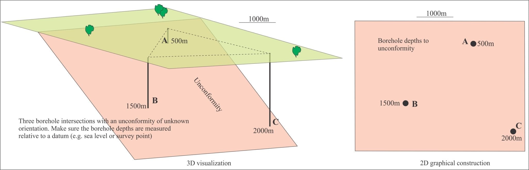
The orientation of geological planes in the subsurface is no less important than in surface mapping, but the database is commonly one-dimensional (e.g. borehole depths and lithologies). For example, a zone of mineralization at depth lies beneath an unconformity; knowing the orientation of the unconformity plane will give us more confidence predicting the trend of mineralization (assuming the unconformity is reasonably flat). To solve the problem, we need depths from three borehole intersections with the plane. The solution is commonly referred to as the 3-point problem. It is based on an understanding of dip and strike.

Geometric calculation of dip and strike in a 3-point problem

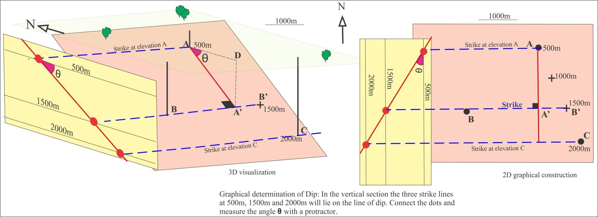
A graphical solution is shown in the animation. You need paper, a ruler and a protractor. This method requires the horizontal and vertical (depth or elevation) scales to be the same (no vertical exaggeration). Normally the construction would be done on the plane itself (i.e. 2-dimensional) – here the 3-dimensional view has been added to help you visualize the problem.

The animation was made from still images: use the pause and play buttons as you work through the exercise.