This post is part of the How To… series
Identifying sedimentary structures that indicate paleocurrent directions is an important task in any study of sedimentary rocks. Knowing the direction of sediment transport will help you decipher paleoenvironments and sedimentary facies, paleoslope dip directions, possible sources of sediment, and the location of sediment sinks.
It all begins with a humble crossbed, flute cast, or current aligned object. Identifying any of these is reasonably straight forward; knowing what to measure can be a bit tricky.
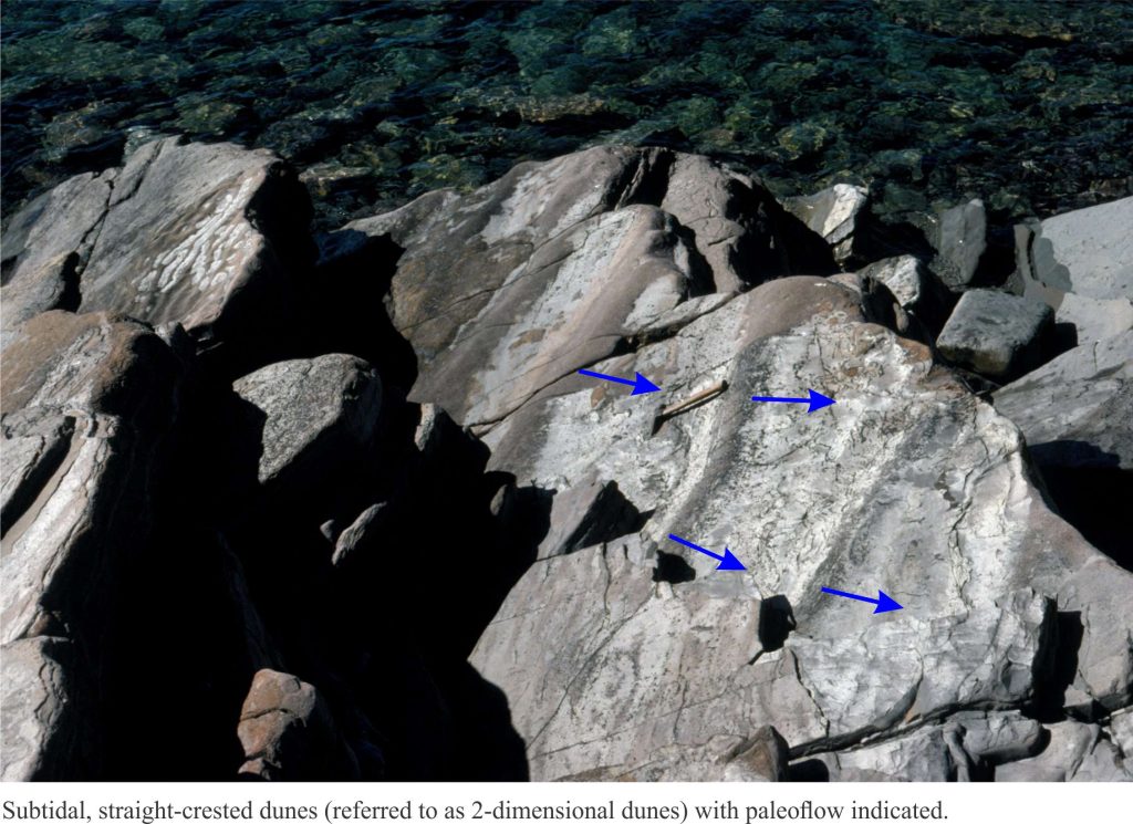
Asymmetric current ripple and dune bedforms exposed on bedding planes can be measured by noting the facing direction of lee slopes (face down current – see the image above). In such cases, measured bearings for individual bedforms provides a unique sense of flow.
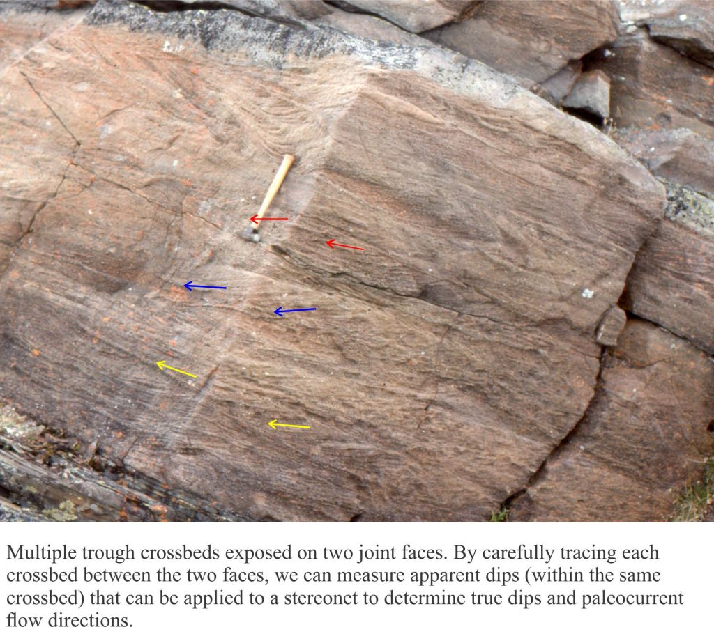
However, it is more common to find crossbed cross-sections in 2-dimensional exposures like cliffs and road-cuts. In situations like this, the crossbed foresets are more likely to present an apparent dip direction, rather than true direction of flow. The trick here is to look for nooks, crannies, joint or fracture faces that present a degree of three-dimensionality to the outcrop.
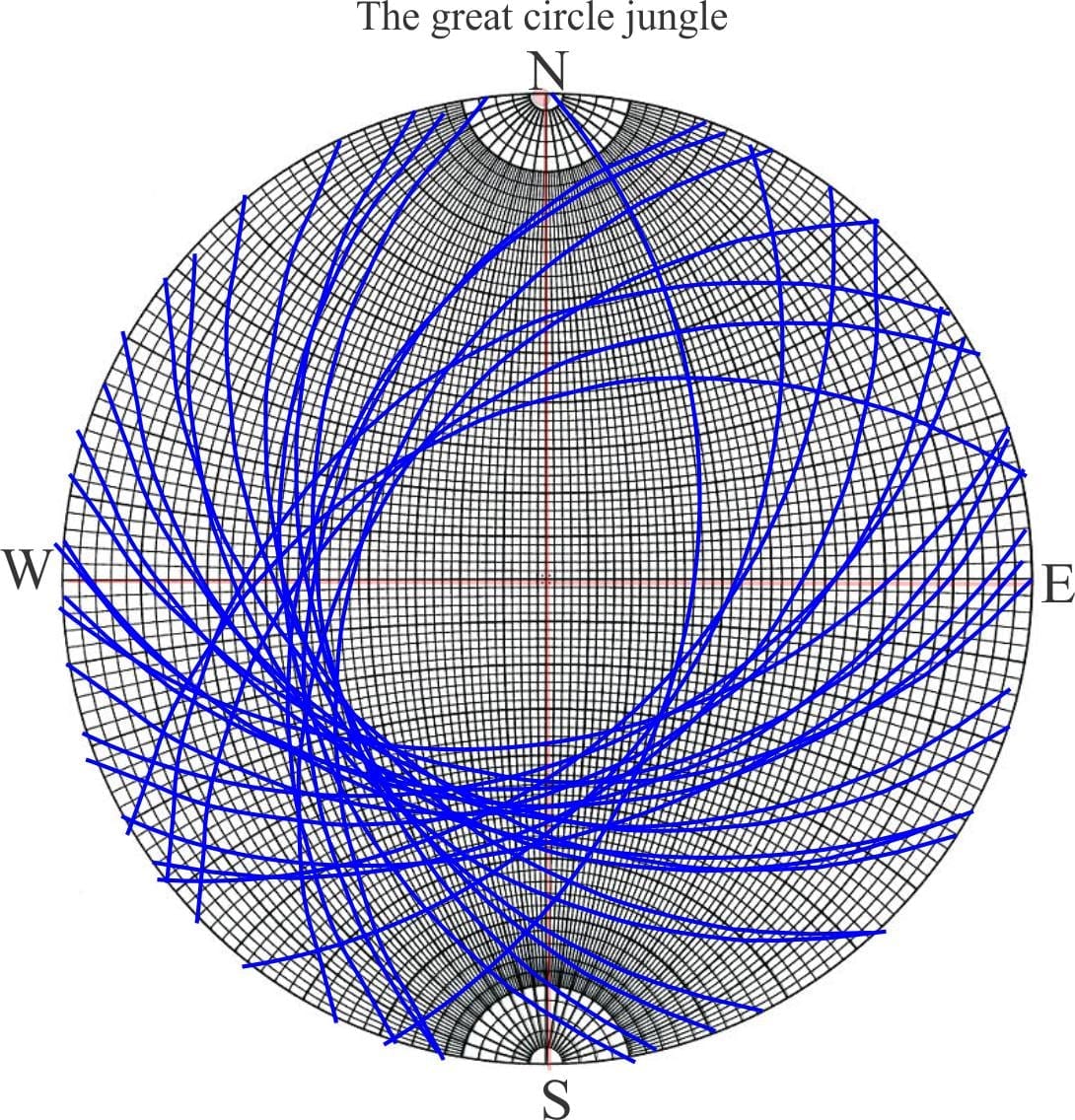
In the example below, crossbed foresets are exposed in two rock faces of a joint block, presenting us with two apparent dips. Measure both plunge and bearings, and find the true dip using stereographic projection. In most cases, the direction of maximum foreset dip will be close to the paleoflow direction. BUT! You must be certain that the foresets belong to the SAME CROSSBED SET. This stipulation is important in situations where multiple crossbed sets cut one another – a feature of sandy fluvial and shallow marine deposits.
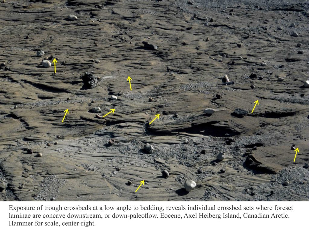
In exposures where crossbeds have been eroded parallel or slightly oblique to bedding, crossbed laminae are outlined in sinuous and festoon patterns. Trough crossbeds, and various 3D ripples exposed in this way (e.g. lunate ripples) provide an opportunity to take multiple paleocurrent measurements. In the example of festooned crossbeds shown here the concave aspect of each trough set faces downstream.
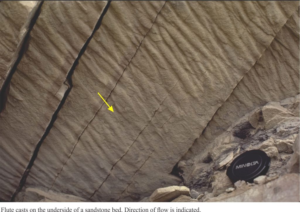
Of all the sole structures, flute casts are the most useful, providing (relatively) unambiguous paleoflow; flow is parallel to the length of the flute, from the deeper spoon-shape scour to the thin feather edge. However, paleoflow determined from groove casts is ambiguous, the two possible directions 180o apart. Data from sole structures is improved if flutes and grooves occur together.
Graphical representation of paleoflow
How you treat the data graphically and statistically depends on the number of measurements at any one locality, and the geographic – stratigraphic distribution of data. A few questions you need to ask are:
- Does the number of data points at each locality warrant separate treatment for each locality, or should the data be lumped into a single point of analysis?
- Is the data distributed over a narrow stratigraphic interval (e.g. 1 or 2 beds, or a single coarsening upward sequence of beds), or a more extensive stratigraphic interval?
- If data from multiple localities or stratigraphic intervals is aggregated, will important variations in paleocurrent trend be represented. For example, if there are local bimodal trends representing tidal ebb and flood currents, will these be ‘lost’ if all coastal data is analysed as a single block of data?
- If mean flow direction is calculated, how useful is this measure of central tendency in the context of the overall spread of paleoflow directions?
- Are corrections needed to account for structural dip?
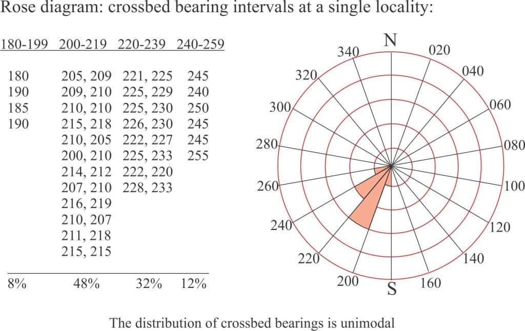
Rose diagrams provide the simplest way of representing data in diagrammatic form. Data is plotted as a circular histogram through 360o. Several software programs are available to do these plots, but it is also a simple task to do it by hand. The inset shows you how to do this.
- With the data in hand, choose a bearing interval (the example here is 20o intervals)
- Organize the data in the intervals and calculate the percentage of measurements for each interval.
- Plot each interval so that the length of each sector of the rose is proportional to the number of measurements for that interval. The example here uses intervals of 20%.
The distribution is clearly unimodal. We could have chosen a 10o or 15o bearing interval for the plot which would probably show some finer detail about the paleocurrents.
Paleocurrent distributions in sedimentary basins generally fall into 3 or 4 categories: Unimodal (one primary direction), bimodal bipolar (2 directions 180o apart), bimodal oblique 2 directions at different angles), and polymodal (widely distributed). Vector means for unimodal distributions are useful for comparing paleoflow among locations and assessing regional patterns of flow. However, the mean directions for strongly bimodal or polymodal distributions may have little real-world value in this context.
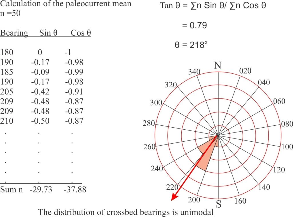
The Mean paleoflow vector can also be calculated, but the usual arithmetic methods DO NOT APPLY to azimuthal data. Calculation of the mean for our unimodal distribution is shown below.
Note: All the bearings are in the SW quadrant and therefore Sine and Cosine values are all negative, and Tangent values are positive. Other distributions may have a mix of positive and negative values – make certain you use the correct sign.
Here are a couple of free Rose plot programs (there are lots of commercial programs available):
GeoRose (free) for Windows and Mac
GEOrient (free for academic users)
Additional posts in this series:
Measuring a stratigraphic section
Identifying paleocurrent indicators
