Sea level. It’s the most common starting point for any kind of elevation measurement, a datum, that for centuries was understood to be an invariant surface. Then some geologists came along and showed that, for eons past, sea level has risen and fallen countless times; coasts were flooded, sea floors exposed. And sea level is still changing, going up in some places, down in others, but on average it is rising; it has been doing this for the last few 1000 years.
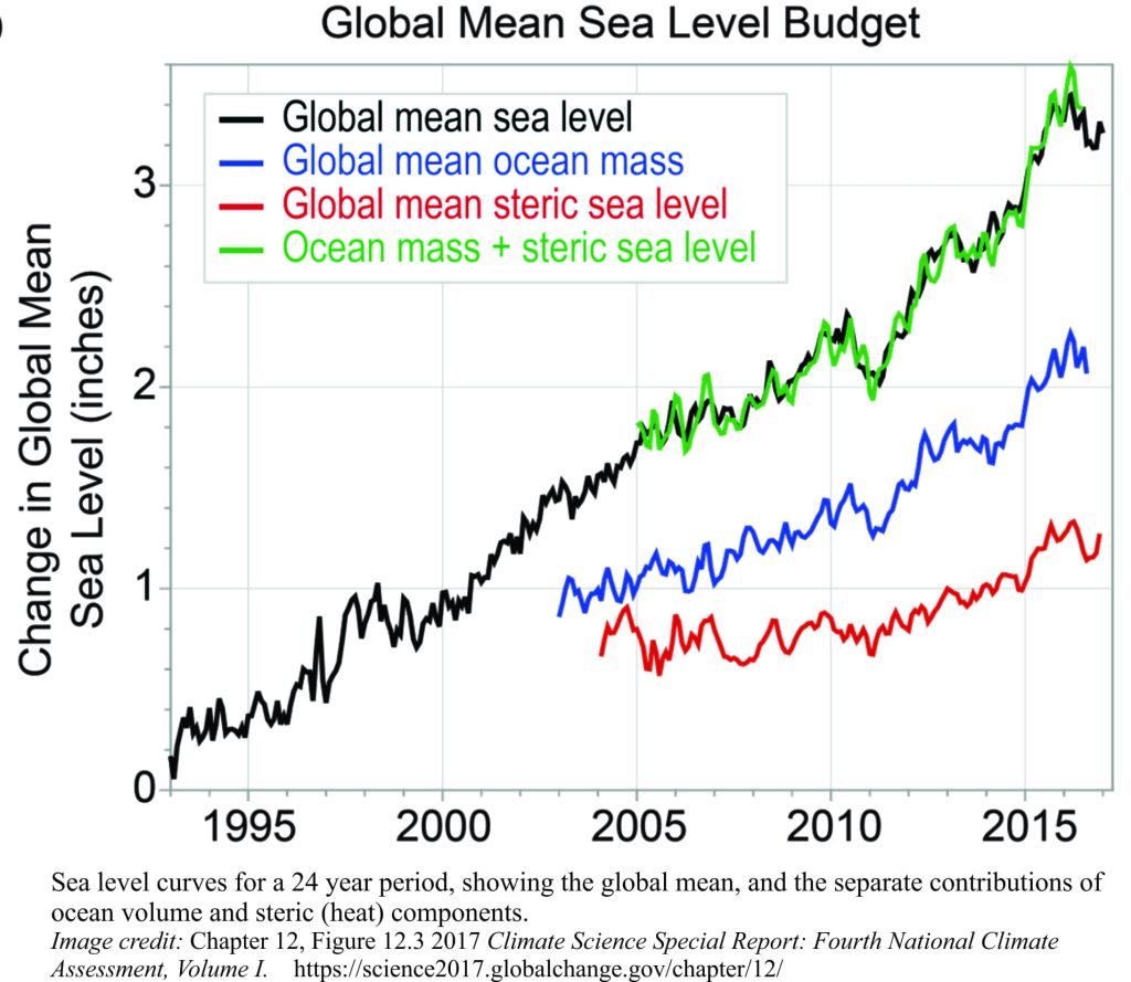
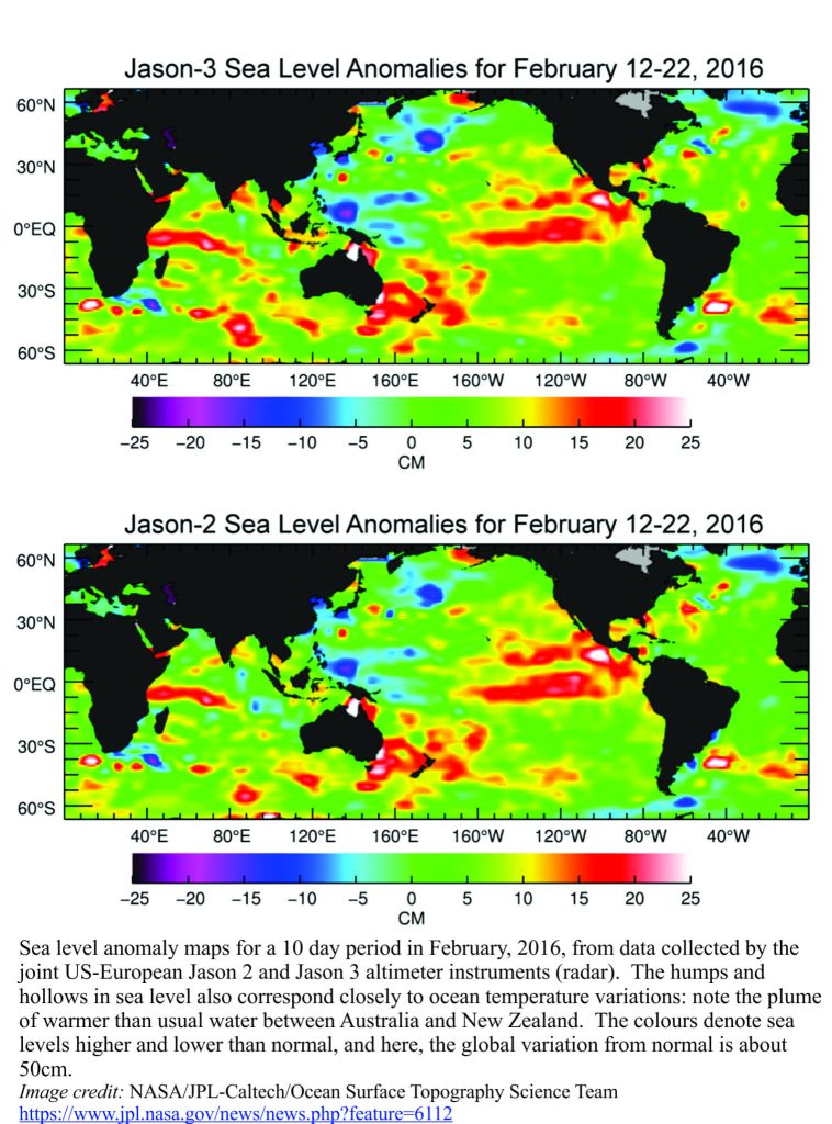
The current globally averaged rate of sea level rise is 3.0 +/- 0.4 millimetres per year, based on satellite altimetry. Satellite measurement of sea level is now about 25 years old. Earlier measurements, some dating back to 1700, were made by tide gauges, basically glorified measuring sticks (the initial technology was just that) which over the years, have become sophisticated, automated measuring systems. Tide gauges measure water levels on a local scale, and in order to make sense of the data in the context of global sea level, all manner of local variables need to be considered: for example, is the location open to the ocean or a sheltered harbour, storm surges, seasonal changes in currents and water mass temperatures, changes in air pressure (sea levels rise during passage of low pressure systems – this is part of the storm surge), and whether the land is rising or subsiding (i.e. local tectonics). In contrast, satellite altimetry gathers data from a much broader swath of the ocean surface. Both Jason 2 and the more recent Jason 3 satellites can cover 95% of the ice-free ocean surface in 10 days. The accuracy of the Jason 3 radar altimeter is currently an impressive 3.3 cm.
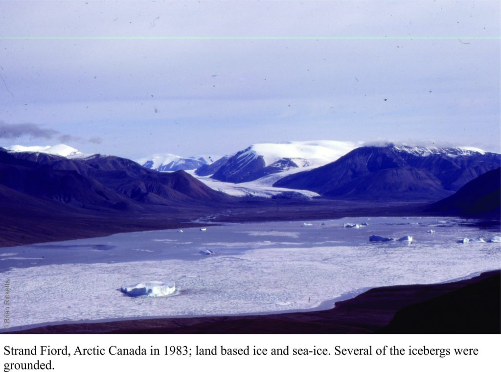
 Rising sea levels and changing climate are inextricably linked because ocean water mass volumes increase or decrease in concert with changes in the volume of land-based ice (primarily the Antarctic and Greenland ice sheets), plus changes in ocean temperature (this is the steric effect) and salinity. Thus, if there is an acceleration in atmospheric warming or cooling, there will be a reasonably sympathetic acceleration in ocean volume change and therefore, sea level change. This is the scenario posited by many climate-change model projections – that increased warming will produce an acceleration in sea level rise. A recent publication that analyses the 25 years of satellite altimetry data (Proceedings of the National Academy of Sciences, 2018), concludes that the (global) average sea level rise is accelerating at 0.084 +/- 0.025 mm/year2, which means that the current speed of sea level rise (about 3 mm/year), will increase year upon year.
The possibility of accelerating sea level rise during the 20th century, based mainly on tidal gauge data, has been debated although most analyses indicated a degree of ambiguity in the data. In fact, a 1990 ICCP report (page 266) concluded there was little concrete evidence at that time for an acceleration, although re-analysis of 20th century tide gauge data, published in Nature (2015) did show a possible accelerating trend. If that analysis is correct, this is the first time such an acceleration has been demonstrated with reasonable confidence from a single data set.
As the published analysis shows, teasing accurate sea level numbers from the satellite data is not a simple task. As is the case for any kind of remote sensing or monitoring, there are data corrections and filters. Some of the corrections include:
- Terrestrial water storage (rivers, lakes, and groundwater); this is necessary because of natural variability in the exchange between land-based water and the oceans,
- Natural variability in land-based ice storage and melting, that adds to, or subtracts water from ocean masses,
- Natural variability in heat exchange between the atmosphere and oceans (the steric contribution to sea level),
- Multi-year cycles such as ENSO (El Niño Southern Oscillation)
- One-off events such as volcanic eruptions that affect regional temperatures because of ash and aerosols; in this case the Pinatubo eruption influence was incorporated into the analysis.
- And the drift in satellite orbits; this variability is much less than that of tide gauges.
The sum of these errors gives the plus (+) and minus (–) value (0.025 mm/year2) that is attached to the overall result – 0.084 mm/year2 (check the open access publication for details). So, if our current rate of sea level rise is 3mm/year, then in 10 years the rate will have increased (accelerated) to 3.84 mm/year, and after 50 years to 7.2 mm/year (almost double the 2017 rate).
Data correction may seem like a bit of a fudge, but it is a critical part of almost every measurement we take, no matter where or what it is; it is part of the process in science that makes data intelligible and coherent. Correcting data is part and parcel of any attempt to isolate causes and effects, as well as determining the kinds of error that are inherent in all measurements. The bottom line in this example, and one that is pointed to by the authors, is that the analysis is preliminary, and that some of the corrections might change as our knowledge of climate and other global systems improves. However, there is confidence that this kind of analysis is on the right track.
