This post is part of the How To… series
The graphical display and statistical analysis of sediment grain size became a popular pursuit of sedimentologists in the 1950s and 60s, particularly those who studied modern sediments. The science of grain size distributions developed in concert with rapidly evolving concepts of sedimentary facies and a more sophisticated approach to interpreting ancient depositional environments. As such, grain size analysis was seen as a possible addition to a sedimentologist’s toolbox. It didn’t quite work out as planned – but that’s a tale for the next blog.
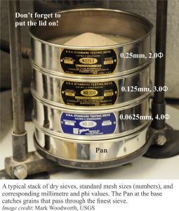
Clast sizes in gravels and conglomerates can be measured directly. For semi- and unconsolidated sands and silts, mechanical sieving is still the preferred method. Wire-mesh sieves are stacked, coarsest mesh on top; mesh sizes are commonly spaced at 1.0, 0.5 or 0.25 phi intervals depending on the range of size classes in your sample. Each sieve will retain sediment that is coarser than the mesh size; grains with a minimum diameter less than the mesh diameter will pass through to the next sieve. A dry sample of known weight is placed in the top sieve and the sieve stack is placed in a mechanical shaker for 10 to 15 minutes. Sieve shakers are notoriously noisy so a sound-proof cupboard is a good idea. Sieve mesh openings range from about 40 microns (4.5ϕ – coarse silt) to 125mm (cobbles). The USGS has a couple of short videos demonstrating this method.
Once shaken, the contents of each sieve are weighed. The cumulative weight from all sieves including the pan should be within 1-2% of the original weight. The weight from each phi interval is converted to a percent of the total weight.
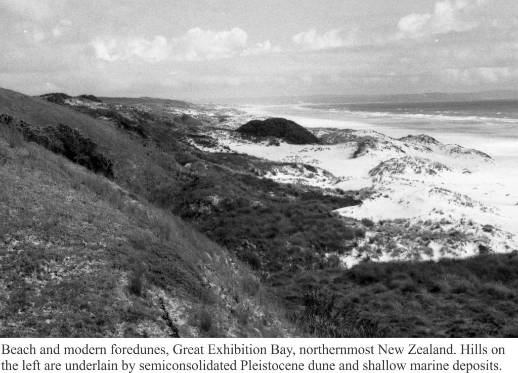
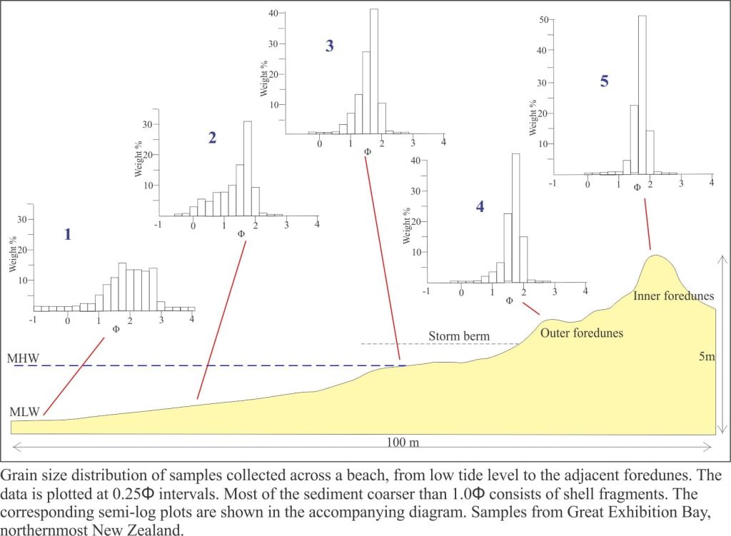
Graphical presentation of the data provides a visual picture of size distribution in each sample and (importantly) the interpolated phi values used to calculate statistical measures. The simplest plot is a histogram of frequency and phi. Examples from modern beach and foredune sands are shown below. The changes in size distribution from low tide to foredunes are nicely represented – there is an obvious (and not unexpected) coarsening towards the high energy surf zone.
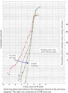
The data can also be plotted on either arithmetic or log templates as cumulative weight percent against the phi values of the corresponding sieve. In most sediments the bulk of the grains tend to cluster round a narrow range of size classes. Log plots emphasize this central tendency and are therefore the preferred graphing method. In the examples below, cumulative weight percents are plotted on the log scale and phi values on the linear x-axis (recall that the phi values themselves are log transformations). Each curve shows a dominant straight-line segment that represents the log-normal distribution of grain sizes for about 95% of each sample. The remaining 5% in the ‘tails’ departs from log normal.
Some basic statistics for each sample can now be calculated: the mean and median grain size (which are measures of central tendency), sorting (that is an expression of standard deviation), and skewness which describes the asymmetry of frequency curves or histograms. The formulae use phi values corresponding to the specified percentile as shown in the diagram above. The most commonly used formulae, developed by R.L. Folk and W. Ward (Journal of Sedimentary Research (1957) 27 (1): 3-26) are:
Median The phi value at the 50 percentile (ϕ50)
Mean Mϕ = [ϕ16 + ϕ50 + ϕ84] /3
Sorting σϕ = (ϕ84 – ϕ16 /4) + (ϕ95 – ϕ5 / 6.6)
Skewness Sk = [(ϕ16 + ϕ84 – 2 ϕ50) /2(ϕ84 – ϕ16)] + [(ϕ5 + ϕ95 – 2 ϕ50) / 2(ϕ95 – ϕ5)]
An additional measure of central tendency is the mode, which is the phi value of the most abundant size class. Note that median, mode, mean and sorting have units of phi; skewness is a dimensionless number.
Median and mode are useful descriptors of sediments but they do not convey as much information about the conditions of deposition as mean and sorting. Mean values represent the most common sizes classes in a sample and may give an indication of the prevalent current strength.
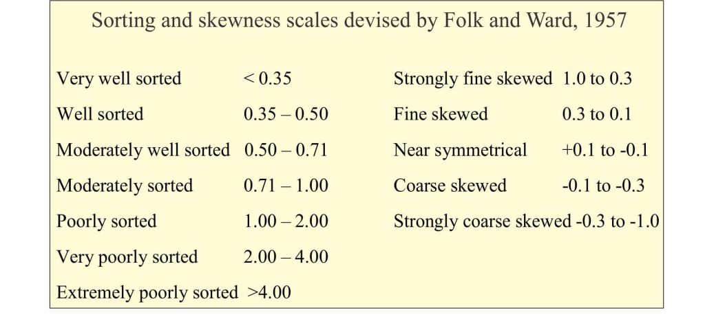
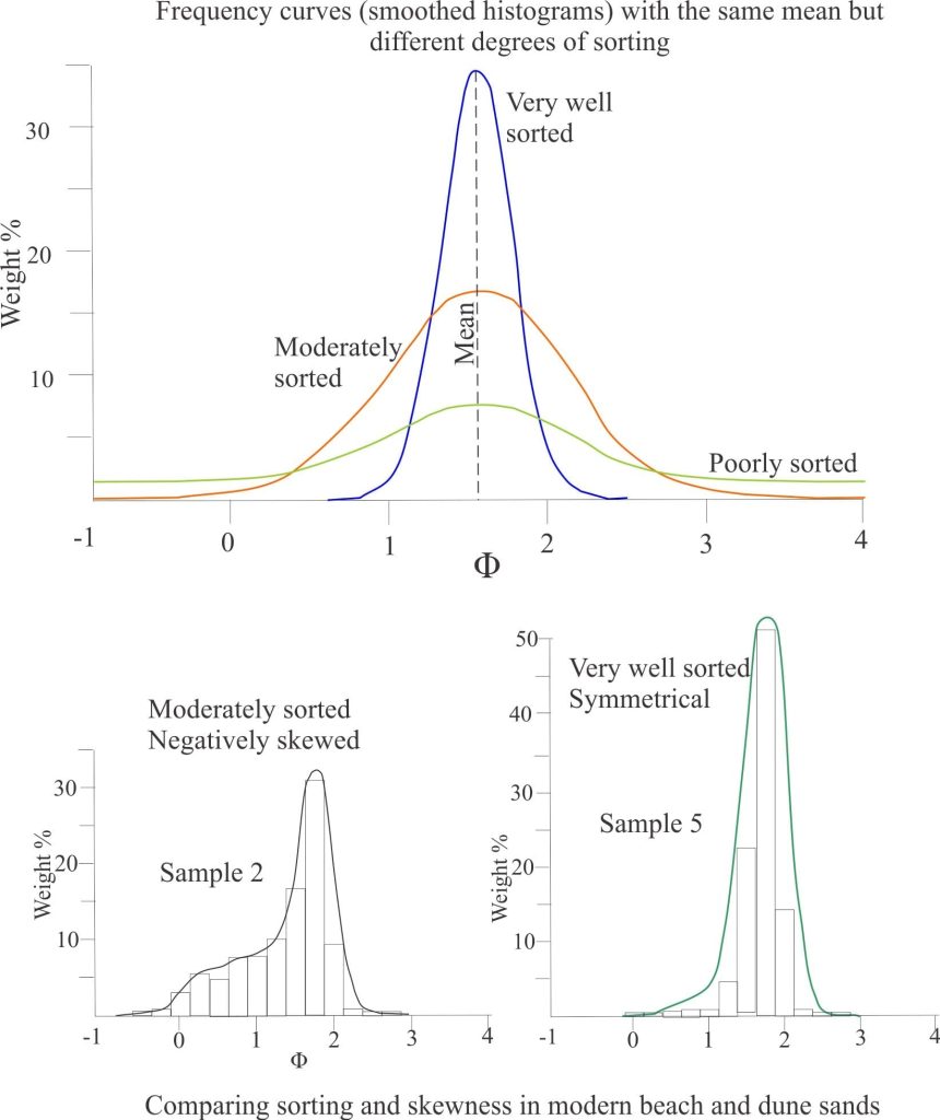
Sorting measures the spread of size classes about the mean. In the beach-foredune example shown above, wind strength is strong enough to move sand but not the coarser shell material that has been selectively removed. Folk and Ward also devised a sorting scale based on calculated phi values.
The foredune and upper beach samples in our example are very well sorted, whereas the lower beach samples are moderately well sorted.
Note that when quoting a mean, it is important to also include the sorting value (standard deviation). The example above shows three samples that have the same mean grain size but clearly are very different sediments.
Skewness describes the symmetry of grain size distributions, or more commonly the departure from a symmetry. Skewness takes the ‘tails’ of the frequency curve into account, such that a surplus of fine material produces a positively skewed histogram (or smoothed curve), and an excessive coarse tail a negative skew – the classification of skewness proposed by Folk and Ward is shown in the chart.
Some other useful links
Crossbedding – some common terminology
The hydraulics of sedimentation: Flow Regime
Describing sedimentary rocks; some basics
Grain size of clastic rocks and sediments





2 thoughts on “Analysis of sediment grain size distributions”
You have the percentiles reversed because the percentage scale (Y) is reversed. Folk & Ward said in the Brazos river article that the 16th percentile is the representation of the coarser part of the sample and the 84th percentile the finest part. Your values will get wrong for reversing these two. It does not affect the mean but surely will affect all the other three statisticals. Here is the original text from Folk & Ward: “Here, the ¢16 may be considered roughly as
the average size a of the coarsest third of the
sample, and the q~84 as the average size of
the finest third; the addition of the q~50
(the average of the middle third) thus
completes the picture and gives a better
overall representation of the true phi mean.”
Thanks, but no.
If you are talking about the semi-log plot, then the % values are plotted correctly – this is standard semi-log graph paper. The 16th percentile identifies the the coarse fraction in all the curves – the green curve about 2.3 phi, the red curve 1.0 phi. The 84th percentile are all smaller grain sizes. Keep in mind that positive phi values are finer grained than negative phi values – because phi is the negative log value.