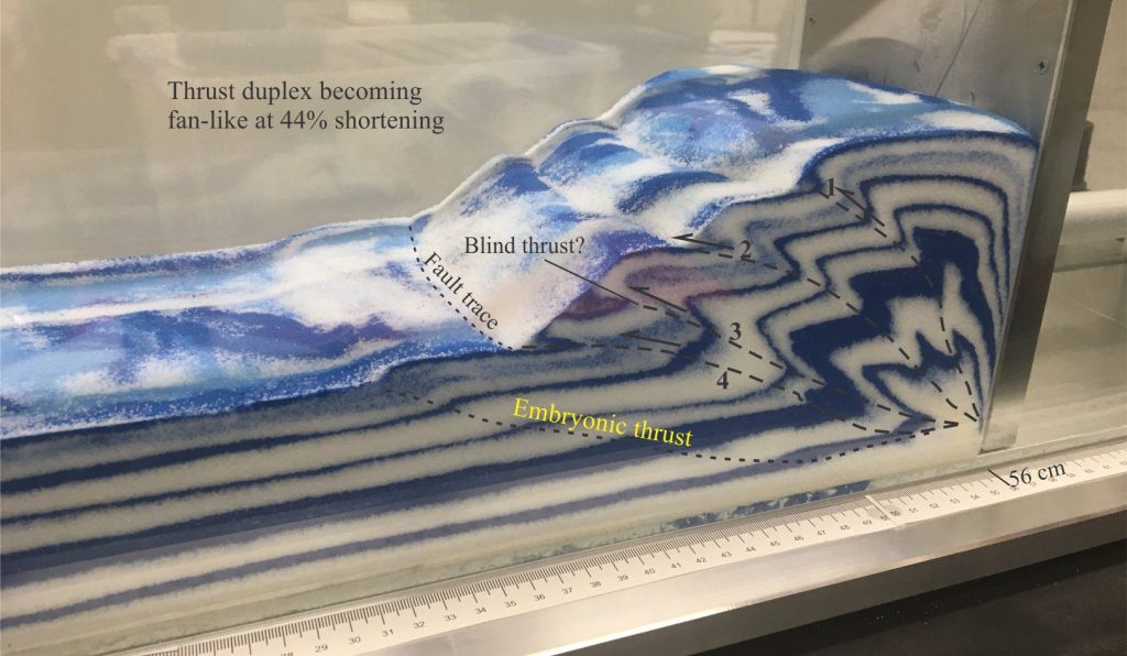
Analogue models are physical objects; we can touch them and observe represented systems directly. As such, they allow us to map the interactions between processes and the physical responses to those processes. Analogue models permit quantitative analysis of a system’s properties.

As noted in an earlier post, the word ‘analogue’ means the correspondence, similarity, likeness, or comparison of one thing to another. Analogies are NOT exact copies of the phenomena in question. Analogies can be observable, theoretical, or conceptual. In Earth science, analogue models are designed to represent some geological system and the processes that govern or control that system. In most cases the systems or objects we want to model are very large – too large and too complex to experiment with directly. Thus, models are scaled-down versions of these systems.

Most analogue models are also scale models where they relate to real world systems by size, geometry, and process, according to some predetermined scale. There are the familiar toys, that are scale replicas of things like ships, dinosaurs, or Barbie-like people. They can be fun to build and to some extent have heuristic value. At a more technical level, wind tunnels and wave tanks are used to observe the aerodynamic or hydrodynamic response of scaled-down versions of planes and ships to fluid flow, turbulence, and waves. Scale models that have figured prominently in geology are those that attempt to unravel the complexities of structural deformation, such as mountain belt folds and fault systems, and the stratigraphic architecture of depositional systems like deltas and fluvial channels.

 

The limitations of analogue models and decision making

Real world dynamic, biological, and chemical systems react in multifarious ways to the large number of variables acting on the systems. It is not the role of analogue models to replicate or duplicate all these system variables. We must decide on a manageable number of variables that can be tested individually or in small combinations, that will answer the questions we have about how the system works. Chris Paola said it best “Simplification is essential if the goal is insight. Models with fewer moving parts are easier to grasp, more clearly connect cause and effect, and are harder to fiddle to match observations (Paola, 2011).

Analogue models have been used in geology for more than two centuries. One of the earliest attempts to model the structural deformation of stratified rock was by James Hall (Royal Society of Edinburgh presentation,1815). Hall initially experimented with layers of cloth compressed laterally between two pieces of wood, the experiments progressing to pliable clay layers in a more sophisticated mechanical box. Horizontal shortening produced folds that Hall considered analogous to those he had seen in the field – notably he had accompanied James Hutton and John Playfair to field exposures in 1788.

A now iconic contribution by M. King Hubbert (1934) was one of the first publications to examine the philosophical and methodological basis for analogue models; his paper changed the rationale of analogue modeling from descriptive to analytical – it still stands as a good introduction to the topic.

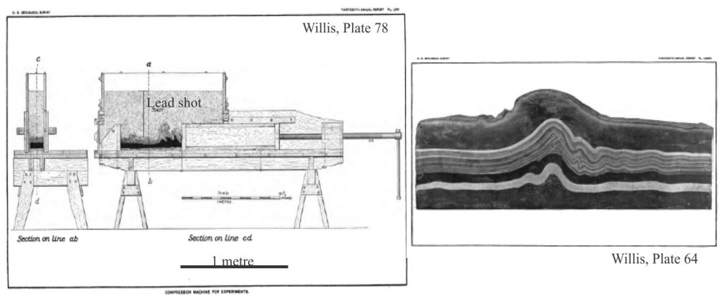
Bailey Willis’ attempts at modeling Appalachian structures serves as a good introduction to the kind of thinking behind the design and execution of the model experiments (Willis, 1894, The Mechanics of Appalachian Structure). The initial questions Willis posed were:

• What is the influence of stratigraphy on deformation (bed thickness, variable bed thicknesses in vertical and horizontal extent)?
• What is the influence of load?
• Is the influence of rock plasticity the same as that as load?

Decisions about the model apparatus and materials that represent layered rock needed to account for (his diagram is reproduced below):

• Changes in the plasticity of the constructed stratigraphy such that it was analogous to the rheology of real strata (Willis used plaster of Paris and waxes).
• Accounting for overburden load (he used a layer of lead shot as a vertical confining load, for which he calculated the pressure applied over the model layers).
• Methods to generate uniform, horizontal compressive stress.
• Recording each experiment as it progressed (photos, sketches – these days we would use videos).

Willis’ methodology also illustrates the central problem faced by all analogue models – how do we scale not only the objects used in the model (their geometry, shape), but the processes we wish to investigate? Willis attempted to reconcile the rheology of the materials used (beeswax, plaster of Paris, and Kerosene) with Appalachian rock properties such as strength (failure limits), but scaling problems meant he had to add an additional layer to act as a burial load. This is illustrated in his experiments where the lead shot layer was required to prevent brittle failure through the top of the layered sequence, but this layer was equivalent to about 160 km of cover rock at the scale he was using. The scale problem is nicely encapsulated by Middleton and Wilcock (1994, p. 83) “The design problem for the model is then to set all the other scale factors so that the model is dynamically similar to the original”. In other words, models must be geometrically, dynamically, and kinematically similar to the real-world systems we are attempting to understand.

Model scaling problems

M.K. Hubbert’s iconic analysis of model scales focused on physical, dynamical systems. One of the first problems we encounter is that scaling of individual variables or quantities is not always linear. For example, if we scale down the measured length of an object by 50%, then the numerical value of the scaled length is obviously half the original length. If, however, we scale volumes by reducing a characteristic length by 50%, the resulting volume is 8 times smaller than the original. If we scale the same length by a third, then the scaled volume is 27 times smaller than the original.

If we now consider the cubes as rock volumes, the mass of each scaled volume will be 8 and 27 times smaller respectively, than the original mass. However, the pressure, or vertical compressive stress exerted by each scaled rock volume on a surface will only decrease by a factor of 2 and 3 respectively.

Hubbert’s lessons in these examples were:

• Variables in dynamic systems can scale differently.
• Dynamical or kinematic analysis of an analogue model will not produce sensible results if the materials used have not been correctly scaled.
• Scaling any variable or quantity requires that the appropriate dimensions are maintained.

Analogue modeling, if it is to be analytically useful (i.e., answering questions) is all about determining the similarity of scaling factors for the important variables that govern processes and their responses – and this is where our problems begin. For his experiments to work, Bailey Willis’ had to add a layer of lead shot over the uppermost model layer – at this experimental scale, the shot layer was equivalent to about 160 km of cover rock which is 3-5 times the thickness of the crust! Thus, Willis’ experiment was qualitatively attractive (i.e., the folds look good) but it could not generate useful data on fold mechanics.

In dynamical and mechanical geological models, we consider scaling similarity in the context of:

• Geometry (characteristic lengths, areas, volumes).
• Kinematics – how do we scale a geological event that takes 10 million years?
• Motion (e.g., velocity, acceleration, direction).
• Forces (e.g., body, surface, elastic, viscous forces).

Scaling geometric quantities is relatively straight forward; scaling models for dynamic and kinematic similarity is not. How do we accomplish this?

 

Model scaling and dimensional analysis

Dimensional analysis and scaling are described briefly in a previous posted article where the procedure is illustrated using the example of fluid pressure drop in a pipe – the analysis results in formulation of the Reynold’s number – an important quantity in any study of fluid dynamics. The result also illustrates the value of dimensional analysis:

• Evaluate the Dimensional homogeneity of equations, where the dimensions must be the same on either side of the equality.
• The dimensions of the numerator and denominator in a ratio must be the same.
• Dimensional integrity must be maintained when converting a variable from one unit system to another system.
• Some quantities are dimensionless. Angular quantities like degrees and radians have no dimensions – they are numbers. All ratios are dimensionless (e.g., porosity, Reynold’s number, Froude number).

Geometric scaling

The geometric scale of a model is expressed as ratios – of lengths, areas, and volumes. For complete similarity, the proportions of each geometric measure for the model must all be the same as the original object or system. The dimensions for each variable must also be the same (in terms of mass M, length L, and time T). Dimensional analysis helps us maintain the correct ratio of dimensions in the ratio numerator and denominator. The simple case for similar triangles is shown below.

The second example has historical significance. We want to find the relationship between the circumference (c) of a circle and its diameter (d). The lengths c and d have a single dimension – L. There are two variables and one dimension [L] and according to the pi theorem, one dimensionless product – c/d or d/c, but the two ratios are reciprocals so in effect there is only one dimensionless product. We can measure both c and d, as folks have been doing since Babylonian times (more than 4000 years ago). Historically the product c/d has precedence – it is the value pi (π); Pi is dimensionless and invariant – its value 3.14159…etc. does not change regardless of the value of d. Note that this is not the same pi as the pi theorem.

 

Dynamic scaling

The same rules apply to the dynamic and kinematic variables of a system. Dimensional analysis provides us with a method to identify the relevant variables and determine appropriate, measurable ratios – these ratios are dimensionless. Critically, the set of ratio products, or pi groups, must be invariant between the model and original object or system for the principle of similarity to apply. Furthermore, for the system being modeled, products in the set must be independent of each other – in other words, each product must not be a multiple of other products in the set. And this is the foundation upon which analogue models should be constructed because the dimensionless quantities remain valid no matter the scale of the model.

A couple of examples.

• Froude number scaling: For any analogue model that investigates the dynamics of fluid flow, the model Froude number must equal the real-world value, which can be written:

(v/√ g.D)_Model = (v/√ g.D)_Real

Because g is the same in the model and the real-world system we can rearrange (and remove the square root):

(v_model / v_real)² = D_model\ / D_real

that allows us to set the scale for both velocity v and water depth D.  For example, if our depth scale is 1/25, then the model velocity should be 1/5 of the real-world velocity, or close to this value if we are to extract answers to questions about the dynamics of stream flow.

 

• Scaling Earth deformation: Scaling deformation at the crustal or lithosphere scale is orders of magnitude different to that in most flume models. There have been many attempts to model Earth deformation, ranging from mountain-scale folds and faults to lithosphere-scale plate tectonic processes such as rifting and subduction. These modeling attempts require establishing a degree of variable similarity between bench-top models (~1 m) and real rifts (10s of km) that means length scaling on the order of 10^-6. Critical variables include stress, rock failure, strain rate, viscosity, density, and gravitational forces. Unlike the flume experiment, inertia can be neglected because rifting proceeds at a relative snail’s pace.

For rift models (Brun 1999, Fort et al., (2004), Smit et al., (2008), and a more recent review by Zwaan and Schreurs (2022), the materials commonly used to represent a layered crust and mantle lithosphere included cohesionless sand (representing brittle rheologies) and silicon putty for ductile regimes. Other products like wet mud and wheat flour have also been used to represent brittle theologies. Silicon putty has also been used in experiments involving salt mobilization and diapirism.

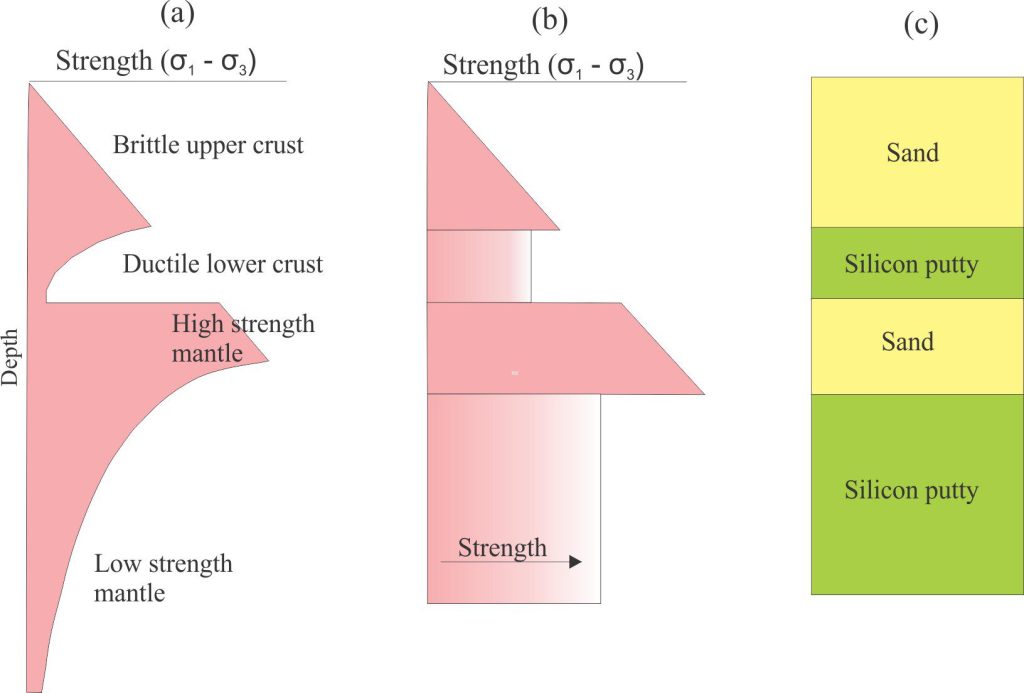
One of the critical scaling relationships is rock strength (a function of σ1 – σ3) that is expressed as model/rift ratios for brittle and ductile layers (the diagram shows a highly simplified lithosphere structure – a necessary simplification to achieve modeling success). For these models it was also determined that the stress ratios and length ratios are approximately equal (~10^-6) (Brun, op cit.) allowing for a more practical approach to model construction. In contrast, the viscosity ratio between ductile crust-mantle lithosphere (viscosity is about 10²¹ pascal seconds) and silicon putty (10³ – 10⁴ pa.s) is on the order of 10¹⁷, which is near impossible to maintain in a model that is measured in 10s of centimetres.

The choice of model material for experiments like these is critical to maintain dynamic similarity in terms of viscosity and density.  A few other materials commonly used in dynamic experiments include (all at 20^oC):

Analogue models have boundaries

All analogue models have physical boundaries. Flumes and sand boxes have a solid base and walls that are essentially impenetrable – there is no sediment or fluid transfer; in dynamic structural models there is no transfer of deformation beyond the walls.

Model walls are necessary, but they can also influence the processes being modeled. For example, fluid flow and sediment dispersal can be deflected in the immediate vicinity of a wall, and in experiments involving deformation, the walls can induce drag. As a general rule, the larger the model, the easier it is to neglect near-field boundary-wall effects.

Boundary conditions also arise from the way in which processes are initiated. The ignition of turbidity currents in flumes commonly occurs with the sudden ‘dumping’ of sediment-water mixtures from a holding tank at the flume head. This determines the initial energy in the flow system and will influence flow momentum (these are energy boundaries). In the same experiments, the dynamics of the density current will also be affected by the degree of initial turbulence in the overlying flume water mass because of drag effects and enhancement of fine sediment elutriation from the turbulent mixture. The initial boundary between density current and overlying water is relatively abrupt, but this changes with the development of an overlying sediment plume behind and above the flow head.

Different boundary conditions are put in place when modeling the effects of gravity on deforming crust or lithosphere. In this case, two popular methods are used:

• A simple sand box where gravity acting on the model is the same as that acting on the real system.
• A centrifuge where compression and extension are generated by centrifugal forces in a rotating apparatus that mimics gravity.

Numerical analyses of the dynamic conditions observed in analogue models also require boundary conditions – in this case to limit the behaviour of numerical functions at model boundaries. Such boundaries may be constant numerical values, such as the rate of subsidence in a model of basin stratigraphy, or a function that defines the rate of change of basin subsidence.

In all cases, boundary conditions, whether physical or numerical, are applied deliberately and systematically because they help constrain the model to a limited number of process variables. In other words, they are important tools used to simplify real world systems so that the models have a better chance of producing sensible results.

 

Other posts in the series on modeling

Geological models: An introduction

Model dimensions and dimensional analysis

Analogue models of faults: scaling the materials

Strike-slip analogue models