How to read a sea level curve

Shallowing upward parasequences in the Jurassic Bowser Basin: each parasequence is a 4th or 5th order cycle superimposed on the regressive stage of a 3rd-order sequence.

Changes in sea level, or baselevel, are central to all forms of genetic stratigraphy. Shorelines migrate basinward or landward because of changes in sea level that we observe in the stratigraphic record as regressions and transgressions. Changes in sea level are caused by eustasy, tectonics, basin subsidence or uplift, or sediment supply, acting individually or sympathetically to create or remove accommodation space. With all these variables potentially operating at the same time, the stratigraphic response to sea level rise or fall can be complicated.

We know that modern sea levels are not the same everywhere because of variations in gravity across Earth’s surface. Furthermore, a change in sea level at one location may not be the same as the change at some distant location because of variations in sediment supply, basin subsidence or uplift, or local tectonic effects that are superimposed on purely eustatic changes. For example, sea level rise that should correspond to transgression, might be offset by high rates of sediment supply resulting in aggradation and even progradation. Thus, the stratigraphy we observe might inform us of trends in water depth or excursions of shorelines but deciphering the actual cause of sea level change is difficult, a conundrum that has occupied the minds of geologists and publication space for decades. We tend to navigate this problem by using the term relative sea level. A cynic might see this as an expression of our collective ignorance, but I prefer to think of it as a pragmatic response to the unknown.

A useful graphical tool to visualize changes in baselevel is the sea level curve. Sea level curves are commonly appended to diagrams that show stratigraphic trends such as shallowing or deepening upward trends, condensed stratigraphic sections, or stratigraphy that contains surfaces of exposure and erosion.

Reading a sea level curve

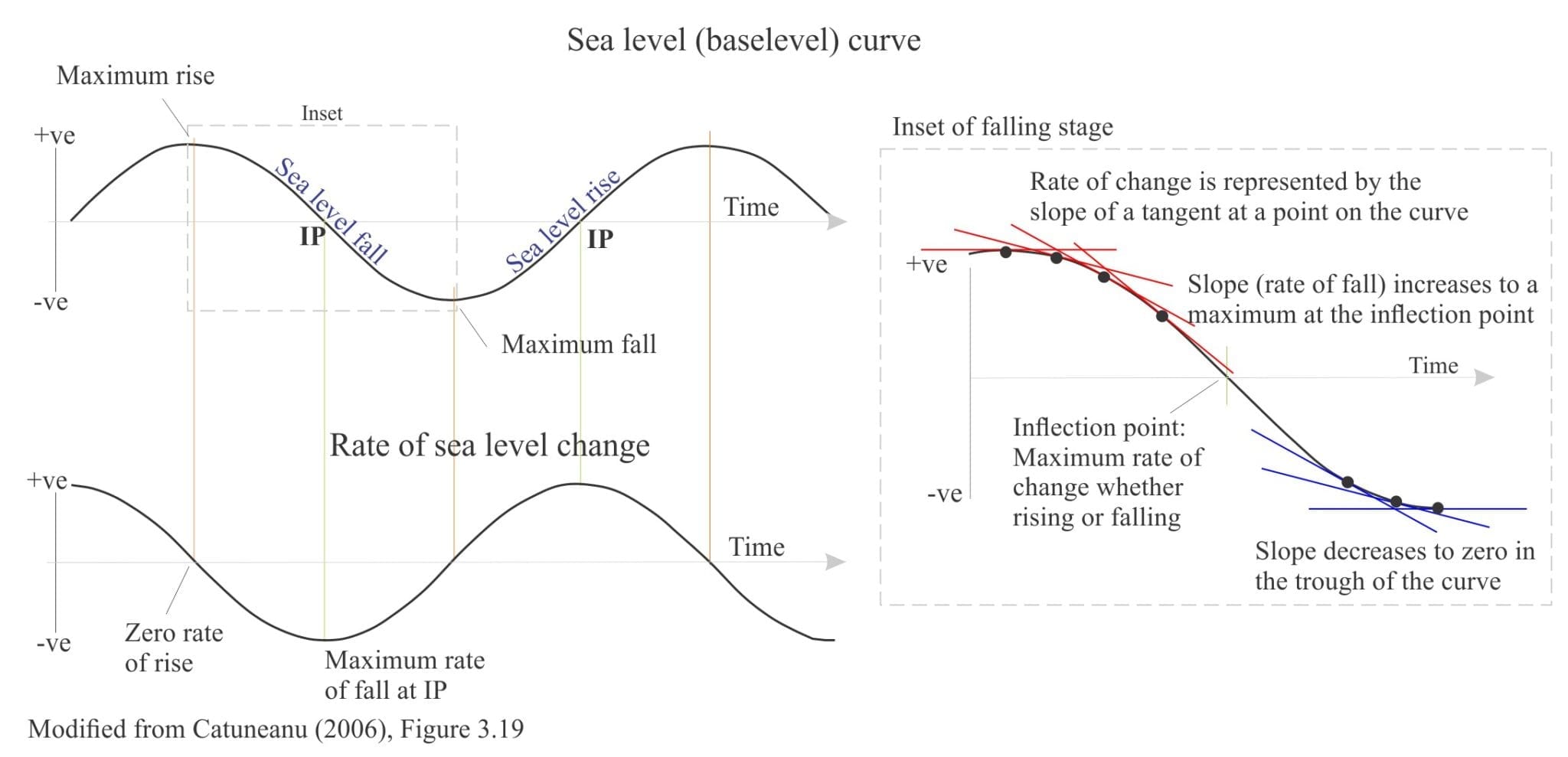
Sea level trends inferred from stratigraphy are usually graphed as sinusoidal curves, with the amplitude of rise (+ve) and fall (-ve) plotted on the y axis, and time on the x axis; Zero sea level corresponds to an inferred shoreline. Curve peaks and troughs measure maximum and minimum sea level changes respectively.

Sea level curves are the graphical representation of amplitude (having dimensions of length) versus time and therefore the gradient of a tangent at any point on the curve will be a measure of the rate of sea level change. This mathematical property means that the curve is a more powerful tool for interpreting stratigraphy than if it was just a measure of actual amplitude. The example above shows the rate of change for a sea level fall segment of the curve. The rate of fall increases from the curve peak where the gradient, and therefore the rate of change is zero, to a maximum at the inflection point, whereupon it gradually decreases to zero in the subsequent trough. Two reasons why rates of change are important are:

The rate of sea level change will be determined by the competing or amplifying effects of eustasy, basin subsidence or uplift, tectonics, and sedimentation rates; any attempt to decipher the relative contribution of each requires us to work in rates of change rather than simple meterage of rise or fall;
Sedimentation rates are an important determinant of stratigraphic trends and stacking patterns, the recognition of which are central to sequence stratigraphy;

Sea level cycle hierarchies

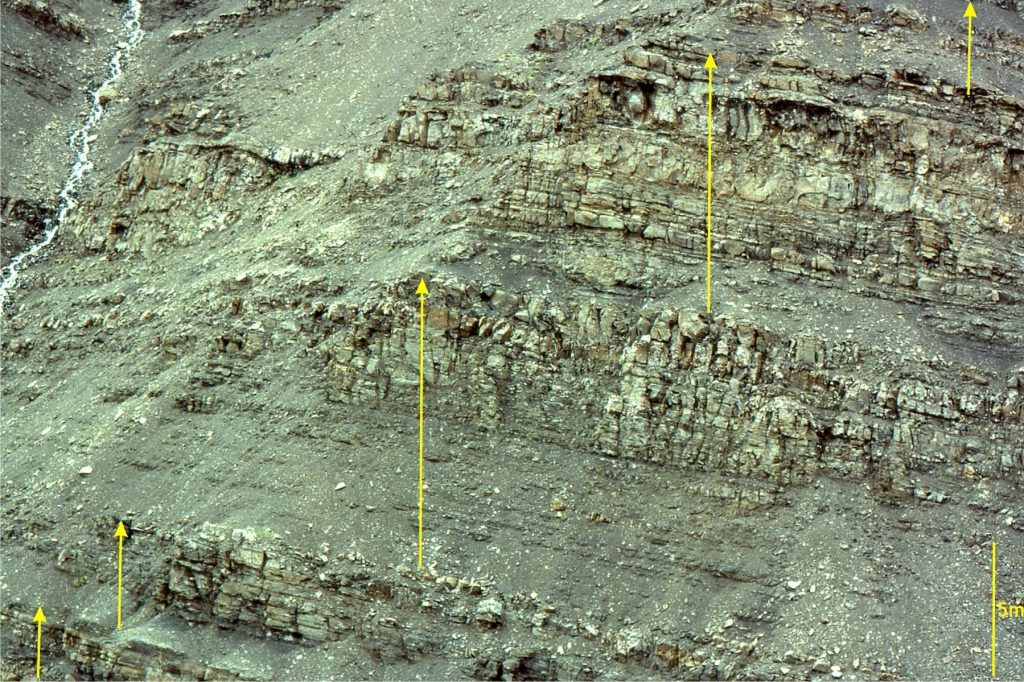
Stratigraphy informs us that there is a hierarchy of cyclical changes in sea level; we see this when comparing rock records from one place to another. For example, at the outcrop we might see a transition in sedimentary facies from muddy shelf to sandy beach – a shallowing upward package of strata where the shoreline has migrated basinward; i.e. a single cycle of relative sea level change. This stratigraphic pattern may be repeated in overlying, successively younger packages of strata. We can visualize this pattern, or trend as a small-scale cycle (outcrop scale) being part of a larger basin-scale cycle.

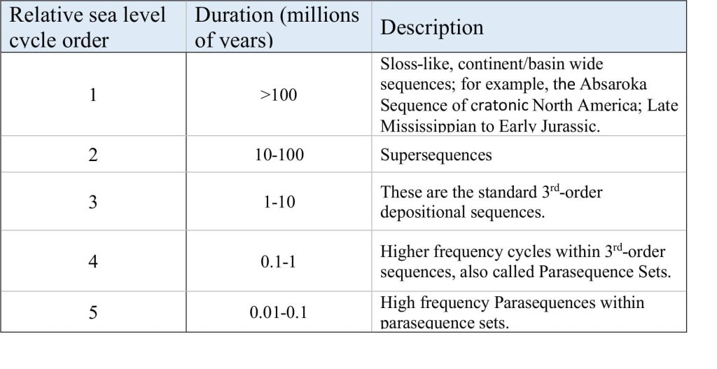
We now recognise five orders of relative sea level cycles, with time frames that range from the life span of ocean basins, to cycles 0.01-0.1 million years duration that are observed at outcrop scale; they are summarized in the list below.

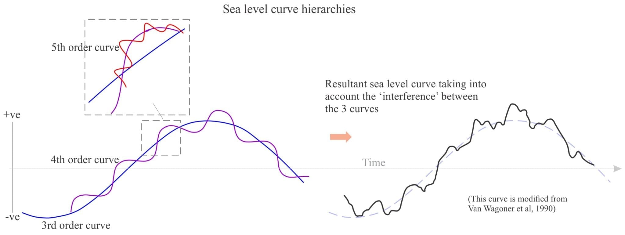
High-order cycles are superposed on lower-order cycles. This is shown schematically in the diagram below. Note that the superposed cycles do not act independently of each other but ‘interfere’. Using an analogy from physics, consider the interaction of waves having different frequencies, such that there is constructive and destructive interference. For example, the rate of rise of a 3^rd-order sea level cycle will be augmented by the rising stage of a superposed 4^th-order cycle, and decreased by the subsequent falling stage. The resulting curve deviates significantly from the smooth, symmetrical 3rd-order sinusoid. Joseph Barrell was one of the first to describe the importance of sea level cycle hierarchies.

Regressions and transgressions

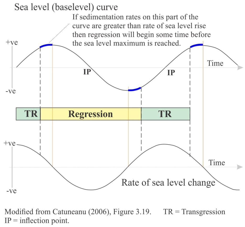
Sea level curves help us to rationalize patterns of cycle stacking in stratigraphy (i.e. stacking patterns). A period of regression at, say, 4th-order scale will result in stratigraphy that indicates progressive shallowing conditions, and a concomitant shallowing upward cycle. Successive 4th-order cycles that are stacked one upon the other will produce the regressive part of a 3rd-order cycle, as shown below. Note however that the regression does not begin (or end) at the sea level curve peak, but at a point on the previous rising stage of the curve. While this may seem counter-intuitive, it is an excellent example of the value of considering rates of sea level change rather than absolute values of amplitude. In this example, the rate of sea level rise slows significantly as the curve peak is approached, and at this stage the rate of sediment supply is sufficiently high to produce regression. The same reasoning applies to transgressions.

This is part of the How To…series on Stratigraphy and Sequence Stratigraphy

References

Barrell, 1917. Rhythms and the measurements of geologic time. Geological Society of America Bulletin v.28, p. 745-904.

Catuneanu, 2006. Principles of Sequence Stratigraphy. Elsevier. 375 p.

J.C. Van Wagoner, R. M. Mitchum, K. M. Campion, and V. D. Rahmanian, 1990. Siliciclastic Sequence stratigraphy in Well Logs, Cores and Outcrops: Concepts for High-Resolution Correlation of Time and Facies: AAPG Methods in Exploration Series No. 7, 55 p. Figure accessed here